Gerd Heber and Joe Lee, The HDF Group
| Editor’s Note: Since this post was written in 2015, The HDF Group has developed HDF5 Connector for Apache Spark™, a new product that addresses the challenges of adapting large scale array-based computing to the cloud and object storage while intelligently handling the full data management life cycle. If this is something that interests you, we’d love to hear from you. |
In an earlier blog post [3], we merely floated the idea of bulk-processing HDF5 files with Apache Spark. In this article, we follow up with a few simple use cases and some numbers for a data collection to which many readers will be able to relate.
If the first question on your mind is, “What kind of resources will I need?”, then you have a valid point, but you also might be the victim of BigData propaganda. Consider this: “Most people don’t realize how much number crunching they can do on a single computer.”
“If you don’t have big data problems, you don’t need MapReduce and Hadoop. It’s great to know they exist and to know what you could do if you had big-data problems.” ([5], p. 323) In this article, we focus on how far we can push our personal computing devices with Spark, and leave the discussion of Big Iron and Big Data vs. big data vs. big data, etc. for another day.
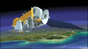
As our reference data set we chose the GSSTF_NCEP.3 [2] collection from NASA’s MEaSURES project. It is a reprocessed satellite data product, which provides a uniform data set of sea surface turbulent fluxes and is useful for global energy and water flux research and applications. It consists of 7,850 HDF-EOS5 files covering the period from 1 July 1987 to 31 December 2008. Each file is around 16 MB, bringing the total to about 120 GB.
The experiments in this article follow the same pattern: We use a driver script, which reads a dataset of interest from each file in the collection, computes per-file quantities of interest, and gathers them in a CSV file for visualization. [6]
The driver script is very similar to the script in [3]. It recognizes up to two arguments (lines 10-11), a base directory to search for HDF-EOS5 files (mandatory) and the number of partitions to create (optional, default: 2). For this example, we have hardcoded the HDF5 path name of the 2-m air temperature dataset (line 14).
1  import os, sys
2  import h5py, numpy as np
3  from pyspark import SparkContext
4
5  if __name__ == "__main__":
6      """
7      Usage: doit  [partitions]
8      """
9      sc = SparkContext(appName="GSSTF_NCEP.3")
10     base_dir = str(sys.argv[1]) if len(sys.argv) > 1 else exit(-1)
11     partitions = int(sys.argv[2]) if len(sys.argv) > 2 else 2
12
13     # the dataset to be explored
14     hdf5_path = "/HDFEOS/GRIDS/NCEP/Data Fields/Tair_2m"
15
For each HDF-EOS5 file, a function f will be invoked, which calculates quantities of interest and emits one or more key/value pairs to be included in a Spark RDD. The argument x is a comma-separated string and consists of the file name and an HDF5 path name.
16 #############################################################
17
18     def f(x):
19         a = x.split(",")  # split the string
20         file_name = a[0]
21         h5path = a[1].strip()
22
23         with h5py.File(file_name) as f:
24             dset = f[h5path]  # create a dataset proxy
25
26             # do something with the data
27
28             # return (key, value) pairs
29
30 #############################################################
31
Given a base directory (in line 10), the script generates a Python list of HDF-EOS5 files in lines 33 – 36. The collection contains XML files and other files and we need to filter out the HDF-EOS5 files by their .he5 file extension.
32     # traverse the base directory and pick up HDFEOS files
33     file_list = filter(lambda s: s.endswith(".he5"),
34                        [ "%s%s%s" % (root, os.sep, file)
35                          for root, dirs, files in os.walk(base_dir)
36                          for file in files])
37
We then use the Spark context’s parallelize method to create an RDD with the desired number of partitions (lines 39 – 40).
38     # partition the list
39     file_paths = sc.parallelize(
40         map(lambda s: "%s,%s"%(s, hdf5_path), file_list), partitions)
41
As in [3], the RDD’s flatMap method is our main workhorse, which transforms the file list RDD by executing a function f for each element and by collecting the results in a new RDD. (Later in this article, we show two example functions.)
42 # compute per file quantities of interest
43 rdd = file_paths.flatMap(f)
44
Finally, we write the results to a CSV file.
45     # collect the results and write the time series to CSV
46     results = rdd.collect()
47
48     with open("results.csv", "w") as text_file:
49         # write results to CSV file
50
51     sc.stop()
Assuming the script is saved as doit.py and the HDF-EOS5 files are stored in subdirectories of GSSTF_NCEP.3 in the current working directory, one can invoke the script via:
spark-submit[.cmd] doit.py GSSTF_NCEP.3 4
This will split the file set into four partitions. (The default is 2, if you leave out the last argument.)
Setup
The numerical (non-scientific!) experiments described below were run on a Lenovo ThinkPad X230T with the following configuration:
- Intel Core i5-3320M (2 cores, 4 threads), 8GB of RAM, Samsung SSD 840 Pro
- Windows 8.1 (64-bit), Apache Spark 1.3.0
We downloaded 3.5 years of data: July-December 1987, 1988, 1998, 2008 (a total of 1,281 files). This corresponds to one eighth of the available data, i.e., running against the full collection shouldn’t take more than ten times the figures reported here. In our examples, we only read the 2-m air temperature data sets. Each Tair_2m dataset consists of 720 x 1440 single-precision floating-point values and is stored as an HDF5 dataset with contiguous layout. The datasets can be easily compressed with h5repack, which reduces the file size to about a third of the original size. (We ran h5repack -L -l CHUNK=32x64 -f GZIP=6 .) In our experiments, we did not see a significant change in performance as a result of compression. The disk utilization dropped slightly, but the added CPU load (due to decompression) didn’t help an already pegged CPU. In a CPU-rich and I/O-limited production environment, we would expect substantially better performance.
Summarization
In our first example, we show how to calculate daily summary statistics. For each file, the summarize function calculates the number of samples (non-fill value pixels), the mean, the median, and the standard deviation of the Tair_2m dataset.
1  def summarize(x):
2      """Calculates sample count, mean, median, stdev"""
3      a = x.split(",")
4      file_name = a[0]
5      h5path = a[1].strip()
6
7      with h5py.File(file_name) as f:
8          dset = f[h5path]
9          tair_2m = dset[:,:]
10
11         # mask fill values
12         fill = dset.attrs['_FillValue'][0]
13         v = tair_2m[tair_2m != fill]
14
15         # file name GSSTF_NCEP.3.YYYY.MM.DD.he5
16         key = "".join(file_name[-14:-4].split("."))
17         return [(key, (len(v), np.mean(v), np.median(v), np.std(v)))]
The argument x is a comma separated string of the HDF-EOS5 file name and the dataset name, and is split in lines 2-4. The NumPy module has all the functions (mean, median, std) needed in this example (line 15). However, before calculating statistics the fill values in the dataset need to be masked (lines 9-11). After writing the output into a CSV file, it can be plotted as a daily mean/median time series (see Figure 1).
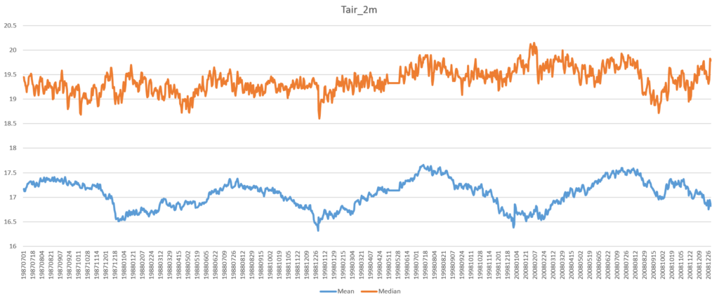
There are a few oddities in this plot, with the plateau between May 12 and May 31, 1998 (see Figure 2) being the most obvious.
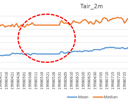
It turns out that, due to a processing error, the data files were written with identical temperature datasets for that period. On the downside, this confirms that we all make mistakes (and will continue to do so). On the upside, with Spark, sanity checks have just gotten a lot faster and cheaper, and everybody can help! (The processing power in your next cellphone will suffice.)
The processing time on our reference machine for 3.5 years of data using 4 logical processors was about 10 seconds.
Filtering
In our second example, we turn to determining the daily top 10 hottest and coldest locations in the data (not on the planet!). This use case is more CPU intensive, since it involves sorting the daily datasets. It is the lazy solution and definitely not practical for larger datasets, but works reasonably well for this example. The top10 function shown below extracts the top and bottom 10 temperatures and locations.
1  def top10(x):
2      """Extracts top and bottom values/locations of Tair_2m"""
3      a = x.split(",")
4      file_name = a[0]
5      h5path = a[1].strip()
6
7      with h5py.File(file_name) as f:
8          dset = f[h5path]
9          cols = dset.shape[1]
10         tair_2m = np.ravel(dset[:,:])  # flatten the array
11         pos = np.argsort(tair_2m)  # indices that would sort
12
13         # offset the minimum by fill values count
14         fill = dset.attrs['_FillValue'][0]
15         offset = len(tair_2m[tair_2m == fill])
16
17         results = []
18         for p in pos[offset:offset+10]:  # bottom 10
19             results.append((p/cols, p%cols, tair_2m[p]))
20
21         for p in pos[-11:-1]:  # top 10
22             results.append((p/cols, p%cols, tair_2m[p]))
23
24         # file name GSSTF_NCEP.3.YYYY.MM.DD.he5
25         key = "".join(file_name[-14:-4].split("."))
26         return [(key, results)]
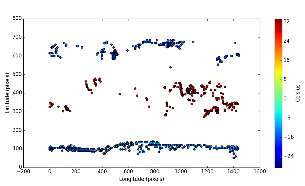
In Figure 3, the distribution of daily minimum and maximum 2-m air temperatures for the 3.5 year period is shown. Pixel (0, 0) is at latitude -90 (South) and longitude -180 (West), and pixel (1439, 719) is at latitude 90 (North) and at longitude 180 (East). With a bit of imagination, one can make out that the lows occur near the poles and the highs around the equator, but this is not a science paper…
The processing time on our reference machine for 3.5 years of data using 4 logical processors was about 50 seconds.
Conclusion
In this article, we have shown a few simple examples of how to use Spark for processing collections of HDF5 files. In a way, we have used Spark as a mere task scheduler and result gatherer. There are other (non-Spark) means to achieve the same, but the simplicity and convenience of using Spark is rather compelling.
Now that we can easily saturate the CPU and disk on a notebook/desktop class machine it might be time to move on and deploy some heavier machinery. Stay tuned…
References
| [1] | HDF-EOS Tools and Information Center |
| [2] | NCEP/DOE Reanalysis II, for GSSTF, 0.25×0.25 deg, Daily Grid, V3, (GSSTF_NCEP), at GES DISC V3 |
| [3] | From HDF5 Datasets to Apache Spark RDDs |
| [4] | h5repack |
| [5] | Harrington, Peter, Machine Learning in Action, Manning Publications, 2012. |
| [6] | https://github.com/HDFGroup/blog |
Good news! The data error we found during this experiment was corrected by the GSSTF team in the latest version of the data product.
Hi Gerd, Nice job for this great innovative idea!!. how many GBs of data read from file to get this results (the mean) in 10 seconds? any performance comparison without spark?
As the article says, we processed only 3.5 years of data (1281 files), and we looked at only one variable per file (Tair_2m). Each grid is 720×1440, but there are a lot of fill values (-999.0). Logically, we read 720 x 1440 x 4 x 1281 bytes (4 -> single-precision floats), or about 5 GB. Note that the execution time does NOT include the Spark startup and shutdown times. Hence, you are effectively looking at a decent SSD read speed. (The computation time is really in the noise.)
We did not compare this to a Spark-free setup. It was really more intended as a ‘kicking the tires’ exercise, and to produce some material for a light-hearted story. We haven’t proven or disproved anything. Even a blind squirrel finds a nut once in a while, and so we came across that processing error in the data…